The initial version of the Imaging Whiteboard had as it’s mission to see if it was possible to perform real-time image processing with a modern desktop PC. The result was a qualified yes.
Since then, its mission has expanded to providing a complete imaging solution; algorithmic processing, frequency domain processing, and neural networks. Version 3.6 including generative AI.
Generative AI has received a lot of attention lately as it has been successful in obvious ways. How much of this success is due to advances in the science, and how much is due to the availability of large datacenters filled with Nvidia chips? Attempting to demonstrate generative AI on a desktop PC might shed some light on this question.
Neural networks date back to 1957 when the perceptron was first invented by Frank Rosenblatt. The same math is still used today. In 1969 Minskey and Papert show how limited a single layer perceptron was. Funding and interest in neural networks declined. In 1974 backpropagation was first described, becoming popular by 1986; this training of multilayer neural networks. In the 1980s Convolutional Neural Networks (CNNs) became practical for handwriting recognition and later computer vision. In 2014 GANs were introduced. By 2022 generative AI was everywhere.
So, how much of this is it possible to reproduce on a PC? A classifier can be trained in a day or two and work fairly well. A generator can be trained in a few hours, but the results are not very good. An Autoencoder can be trained in a couple of days and work reasonably well. GANs cannot be trained in any reasonable amount of time.
It is clear that more performance is required. What do the big-name AI companies do? They use Nvidia chips, lots of them. There is an Nvidia GPU on my PC that does not seem to be doing anything; Managed Cuda is available to enable C++ code compiled to run on the GPU to be called from C#. So, I wrote a couple of small C++ routines to implement backpropagation for a convolutional layer and a fully connected layer, introduced a Use GPU checkbox in the UI, and it ran about 60x slower that the original CPU code!
Timming the various steps in the process, it turns out that the problem is the time taken for the GPU code to execute; not the initial suspects, moving the data into the GPU memory, and the results back out. Double precision floating point numbers do not do well on consumer GPUs. Converting to single precision floating point numbers gave some improvement but not significantly. Turns out that the problem is that I require too few threads to make the GPU efficient. Optimally the GPU should be running 43K threads minimum (at least for the GPU on my machine), my code required at most 18k threads, the CPU will likely always be faster!
So, for now I have to say that training a GAN on a PC is not really a practical proposition; at least not for one man, one PC, and zero budget!
I am looking at other approaches, so this could change.
Now that the Audiophile’s Analyzer is complete how can all of the features be provided to the Musician’s Workbench?
Simply backporting the code would not be the best solution, it would result in massive code duplication. Even more problematic would be the clash of design philosophies.
The Musician’s Workbench was designed to reproduce the functionality of the original SA-10 hardware. It is lean and real-time by design.
The Audiophile’s Analyzer was designed to provide every known music transcription technique, and to provide it all in a single integrated package. It is large and not real time.
The solution is to allow the Audiophile’s Analyzer to import session files from the Musician’s Workbench.
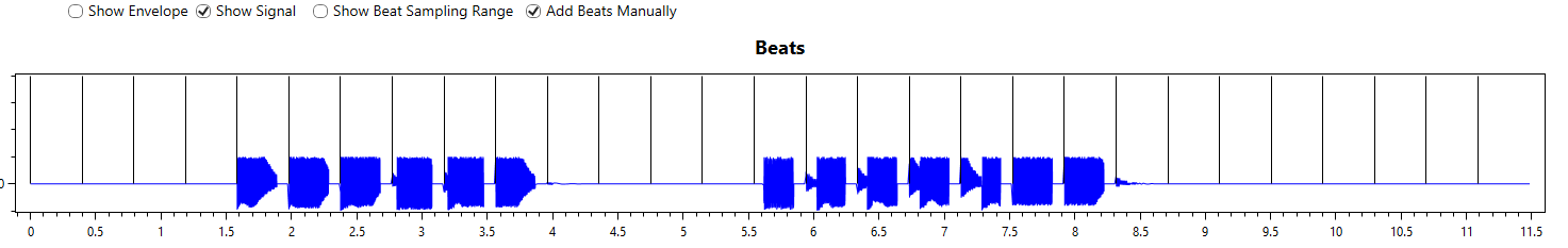
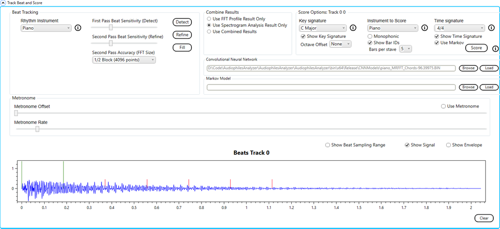
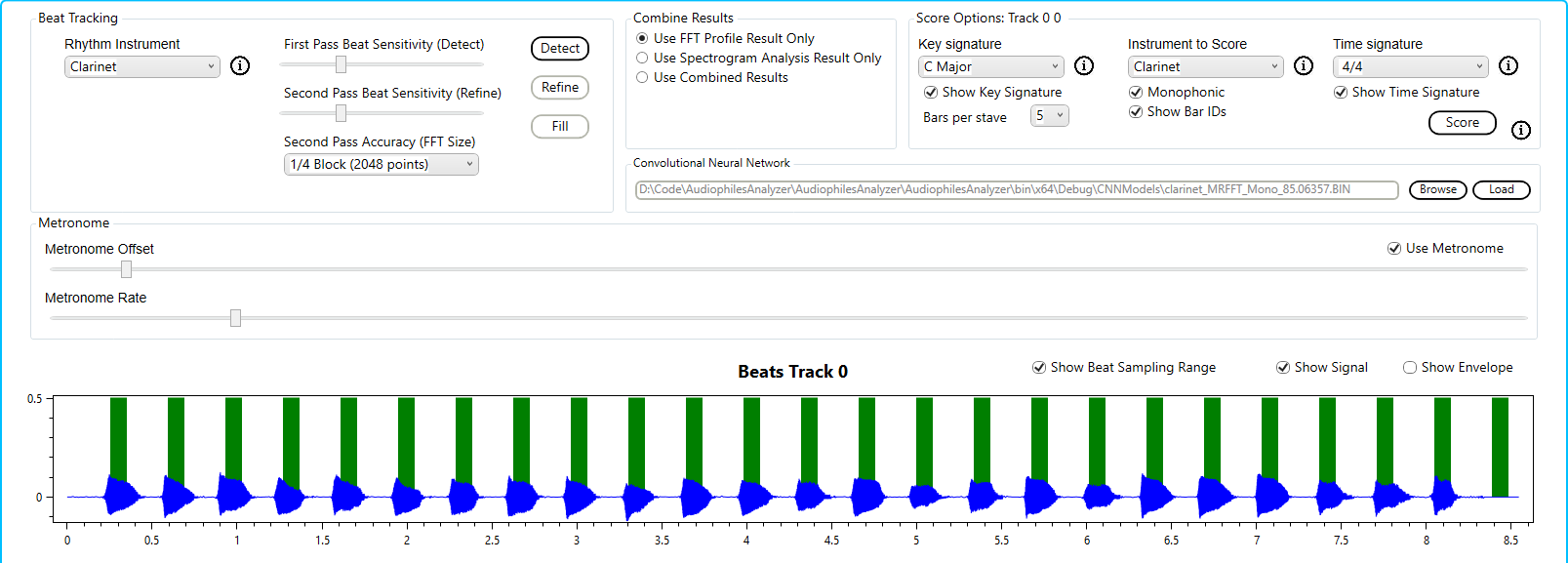
Here we see the Beats graph from the Analysis tab of the Audiophile’s Analyzer. The beats are from the session file, and were originally generated by the metronome of the Musicians workbench. The audio signal is overlaid, this is the original audio sampled by the Musician’s Workbench. The audio was only sampled on the beat when there was sound, and only enough to allow a single FFT to be performed.
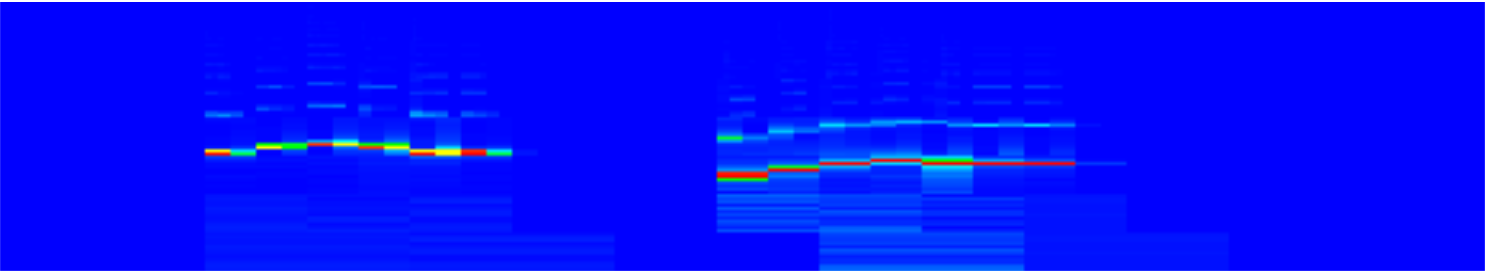
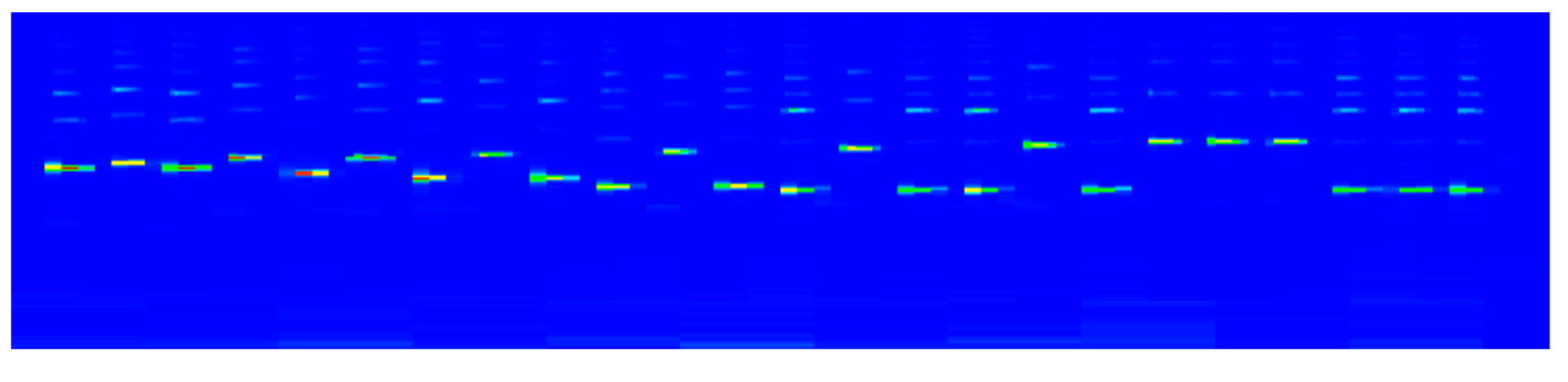
The spectrogram for the same audio is shown.
Now the user can re-transcribe the session using any of the techniques available in the Audiophile’s Analyzer including the built in CNNs. This would simply not be possible in real time as it requires 7 FFTs to be performed before the spectrogram can be sliced and sent to the CNN.
The Audiophile’s Analyzer can also provide some insight into the internals of the Musician’s Workbench which are not normally displayed. Answering questions such as, “Should I have used Delayed Sampling?”, “Did I select the best Octave Range?”.
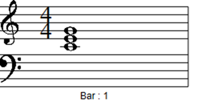
The problem with training neural networks is always finding the training data. Samples of individual notes are available on the internet. Samples of chords are not available.
There are 16 chord types that are recognized by the Audiophile’s Analyzer. There are 96 notes in 8 octaves. So, it is possible to play 1536 different cords on a piano keyboard. It is not practical to play, record and label so many samples.
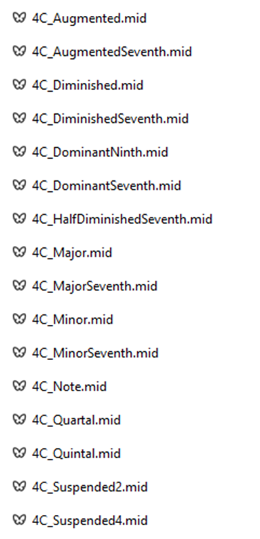
To solve this a feature has been added to the CNN tab of the Audiophile’s Analyzer which will produce MIDI files for every possible chord for a selected instrument.
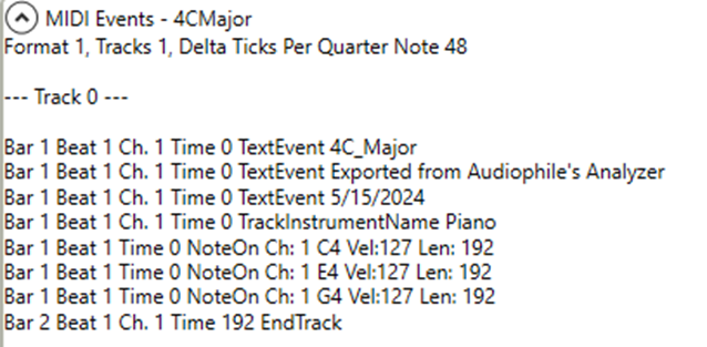
These MIDI files are then converted to .wav audio files using a third-party application. When read by the Audiophile’s Analyzer a spectrogram is produced.
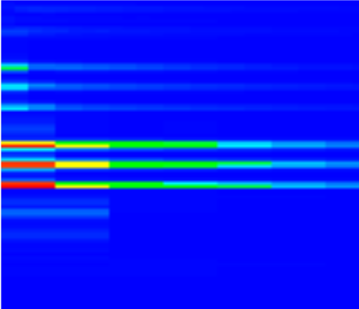
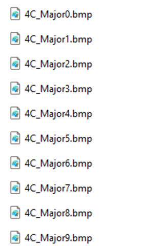
The Training set creation utility is then used to slice the spectrogram to create the training images.
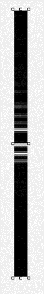
Monochrome images are used to train the CNN, color is for humans.
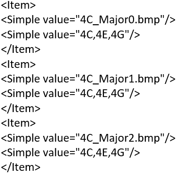
This utility will recognize the filename format and produce the labels file. Multiple labels will be applied to each file.
The Audiophile’s Analyzer is used to build and train a CNN using the labeled images.
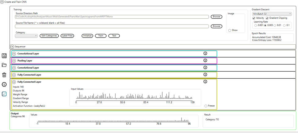
The output layer of the neural network will have 96 outputs, labeled from 0C to 7B. During training the required outputs will be set for each note in the file label.
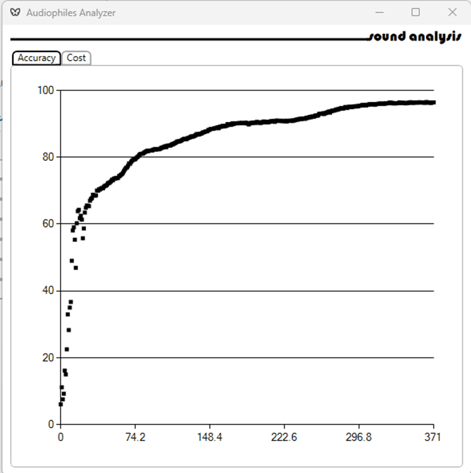
Training results are recorded:
Using the Audiophile’s Analyzer to transcribe a .wav file:
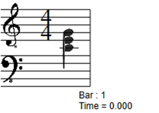
Here I use a sequence of notes played on a clarinet.
The first note is A (octave 4) followed by A#, the final note id E (octave 4).
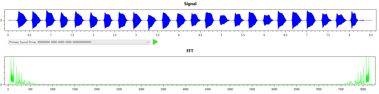
Using the built in profile the correlation algorithm gives:
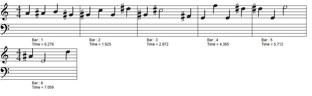
Pretty good.
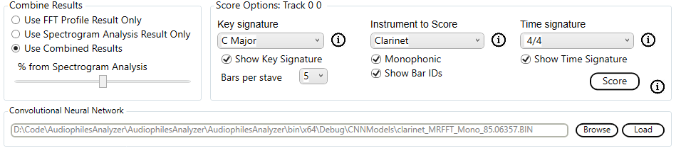
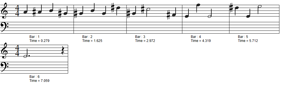
To improve this I used the built in CNN model in combination with the algorithm’s results.
Here I perform the same task, i.e. single note (A2), this time from a cello. This is a little more difficult as the cello is a polyphonic instrument with very strong harmonics.
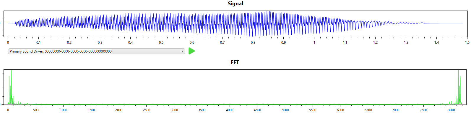
From the signal and FFT result we can see that the first overtone has more energy than the fundamental frequency.

This problem is attenuated in the Multi-rate FFT spectrogram as the overtone is sampled over less time in the shorter sampled higher frequency FFT.
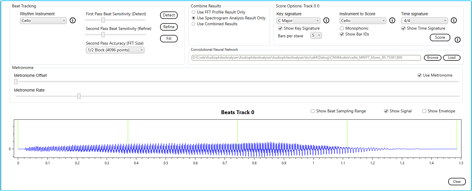
We use the built in profile for the cello.
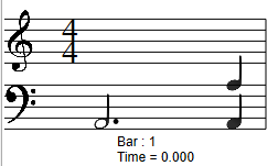
Here we can see that as the note fades on the last beat the overtone is also transcribed.
Since we know that this was a single note the monophonic check box should be checked.
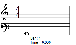
Now the result is as expected.
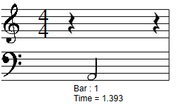
Using the built in Convolutional Neural Network for the cello we see leading and trailing silence; only the red line from the spectrogram has been transcribed.
The threshold for silence is calculated differently for the algorithm and the CNN. The algorithm sets the threshold on the fly during transcription based on a running average of the energy in the audio. For the CNN the threshold for silence is implemented when the spectrogram slices are prepared for training; the CNN was never trained on the parts of the note which were too quiet.
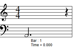
The simplest music file to transcribe is a single note. Here I use a bassoon playing a single note A (octave 2) to walk through the simplest transcription.
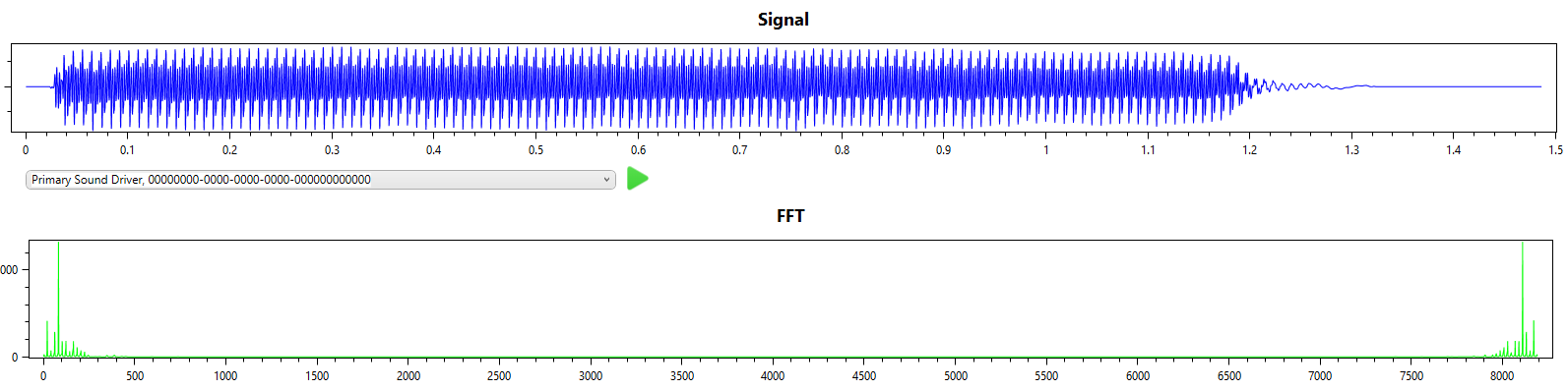
From the signal and FFT result we can see that this is indeed a single note with a single dominant frequency.
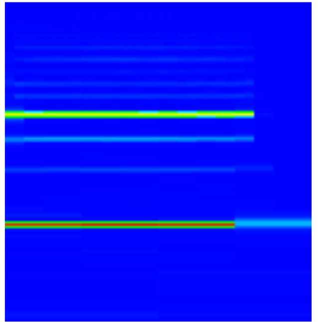
The spectrogram confirms the simplicity of this example.
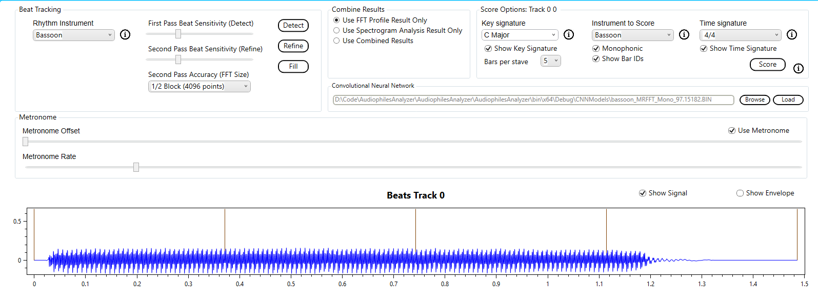
To transcribe this note we will use the built in bassoon profile and the default options (i.e. correlation).
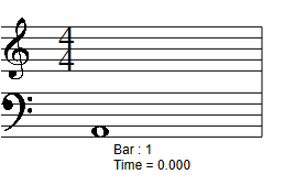
The result is as expected.
Alternatively we could have elected to use the built in Convolutional Neural Network for the bassoon.
The result is a little different. The note ends just after the forth beat. The CNN transcribes this as a 3 beat note, not 4 beats.
Using the MNIST database of handwritten digits MNIST database – Wikipedia a convolutional neural network was trained to an accuracy of 90%. This took 50 epochs.

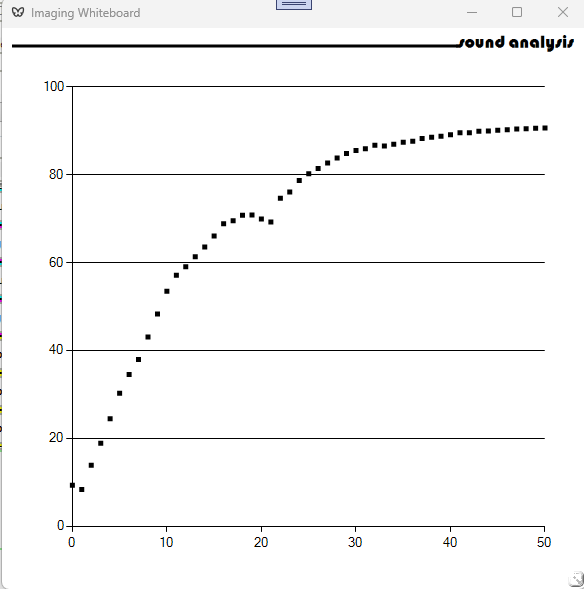
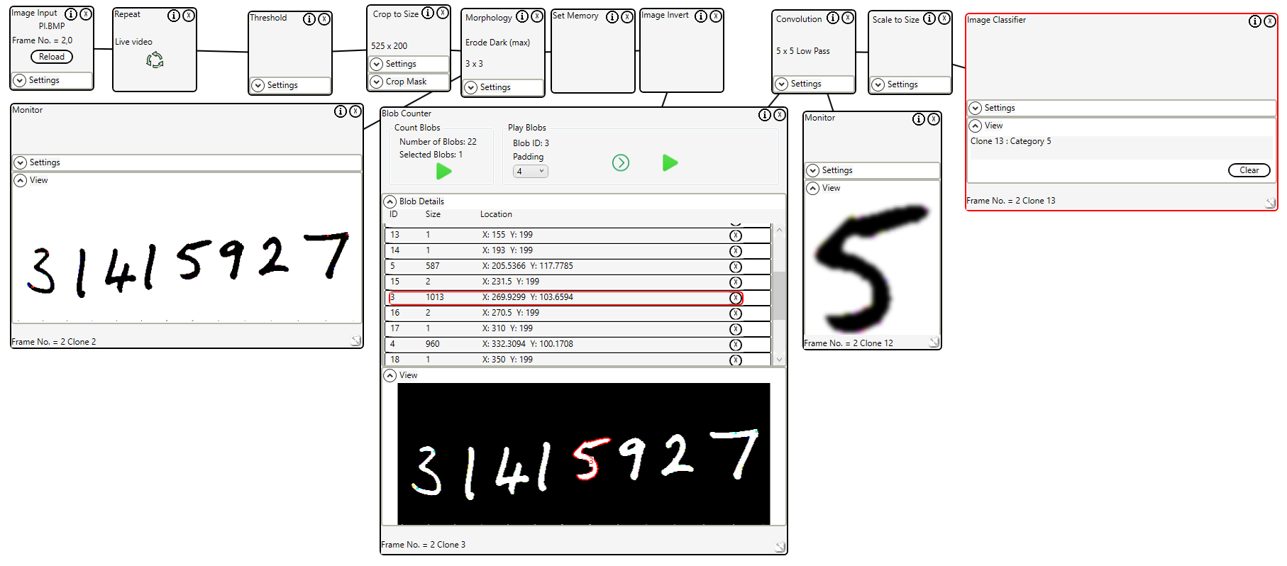
The trained model was loaded into the Image Classifier control and used to identify handwritten digits.
The files required to reproduce this demo are available here https://drive.google.com/file/d/1XKSYvJfAW1maNsaiV0iaWZXor0Tbtuat/view?usp=share_link