The initial version of the Imaging Whiteboard had as it’s mission to see if it was possible to perform real-time image processing with a modern desktop PC. The result was a qualified yes.
Since then, its mission has expanded to providing a complete imaging solution; algorithmic processing, frequency domain processing, and neural networks. Version 3.6 including generative AI.
Generative AI has received a lot of attention lately as it has been successful in obvious ways. How much of this success is due to advances in the science, and how much is due to the availability of large datacenters filled with Nvidia chips? Attempting to demonstrate generative AI on a desktop PC might shed some light on this question.
Neural networks date back to 1957 when the perceptron was first invented by Frank Rosenblatt. The same math is still used today. In 1969 Minskey and Papert show how limited a single layer perceptron was. Funding and interest in neural networks declined. In 1974 backpropagation was first described, becoming popular by 1986; this training of multilayer neural networks. In the 1980s Convolutional Neural Networks (CNNs) became practical for handwriting recognition and later computer vision. In 2014 GANs were introduced. By 2022 generative AI was everywhere.
So, how much of this is it possible to reproduce on a PC? A classifier can be trained in a day or two and work fairly well. A generator can be trained in a few hours, but the results are not very good. An Autoencoder can be trained in a couple of days and work reasonably well. GANs cannot be trained in any reasonable amount of time.
It is clear that more performance is required. What do the big-name AI companies do? They use Nvidia chips, lots of them. There is an Nvidia GPU on my PC that does not seem to be doing anything; Managed Cuda is available to enable C++ code compiled to run on the GPU to be called from C#. So, I wrote a couple of small C++ routines to implement backpropagation for a convolutional layer and a fully connected layer, introduced a Use GPU checkbox in the UI, and it ran about 60x slower that the original CPU code!
Timming the various steps in the process, it turns out that the problem is the time taken for the GPU code to execute; not the initial suspects, moving the data into the GPU memory, and the results back out. Double precision floating point numbers do not do well on consumer GPUs. Converting to single precision floating point numbers gave some improvement but not significantly. Turns out that the problem is that I require too few threads to make the GPU efficient. Optimally the GPU should be running 43K threads minimum (at least for the GPU on my machine), my code required at most 18k threads, the CPU will likely always be faster!
So, for now I have to say that training a GAN on a PC is not really a practical proposition; at least not for one man, one PC, and zero budget!
I am looking at other approaches, so this could change.
I’ve created a channel on YouTube. I’ve posted some short instructional videos to show the basics of the Imaging Whiteboard. There will be more posted soon.
Version 3.5 of the Imaging Whiteboard introduces extended frequency domain processing. The FFT control will now output the FFT results with the output image, a second FFT control will detect the previous results and perform the reverse FFT. Other controls have been extended to support processing these results.
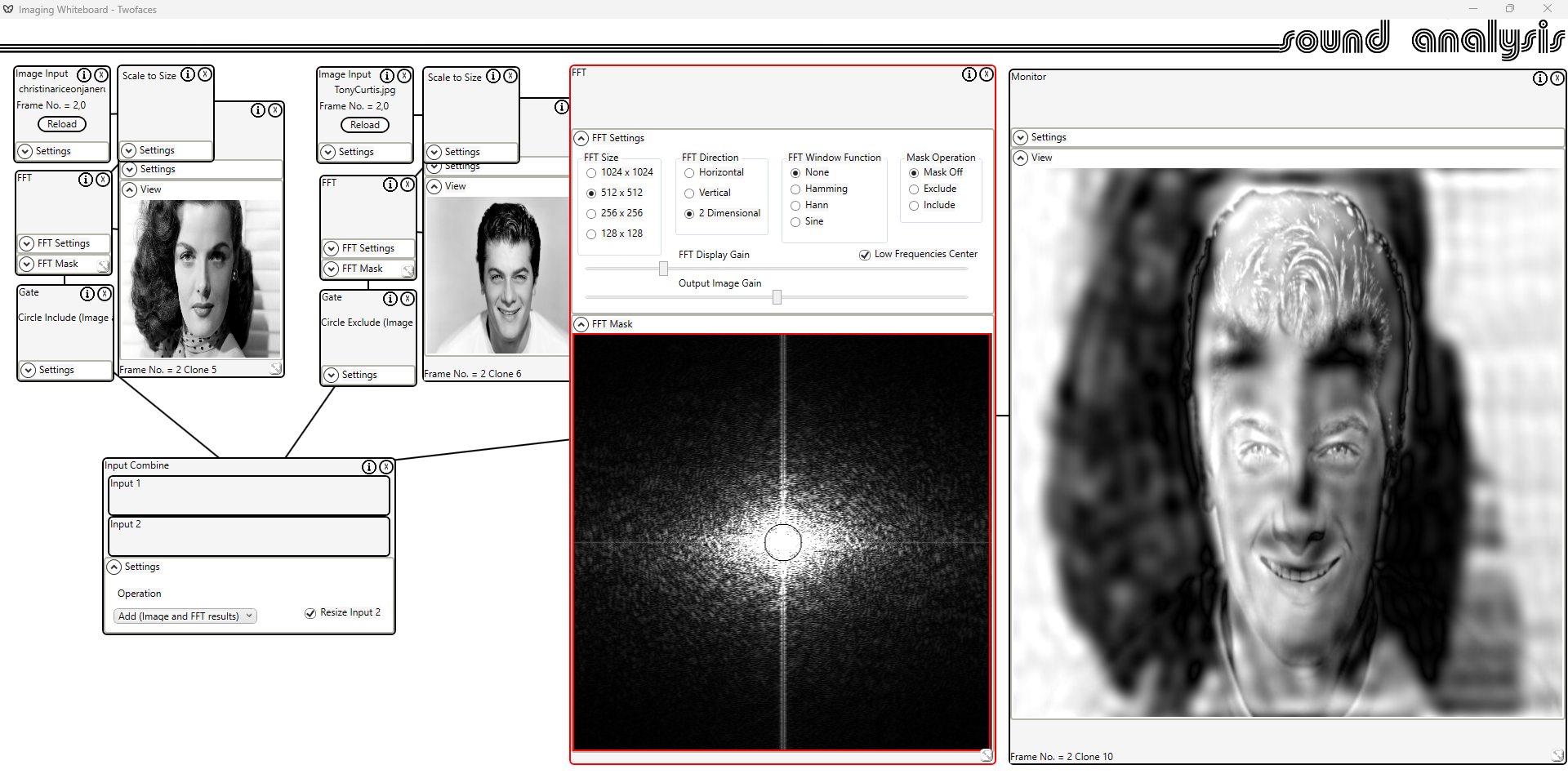
Here an image of Jane Russell has been transformed and the high frequencies excluded. An image of Tony Curtis has been transformed and the low frequencies excluded. The two processed FFT results have been added and the reverse transform performed. When the image is viewed close up the eye sees Tony, from a distance the eye sees Jane.
In the last blog post I showed how the line detector could be used with a Sobel filter. In this post I will show how Canny edge detection https://en.wikipedia.org/wiki/Canny_edge_detector can provide a better input to the line detector.
The latest cookbook http://sound-analysis.com/imaging-whiteboard-3-0/ shows how to use the Line Detector Control with a Sobel filter, and, how to perform Canny edge detection. This post will show how to combine both.
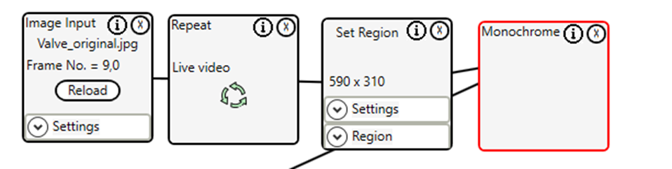
First, we prepare the image; repeat will help making the adjustments to the Canny edge detection, Set region will limit the entire process to a specific region. Monochrome because the Hough transform is a monochrome process.
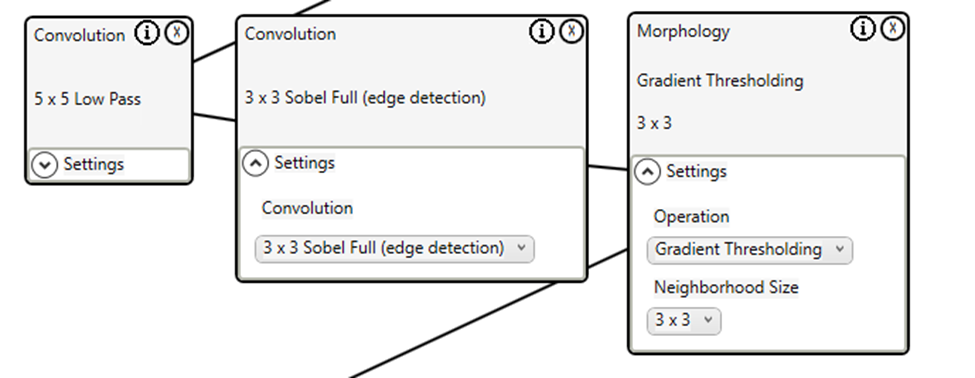
Next, we filter the image to remove noise, and perform the initial edge detection using a full Sobel filter (includes edge direction) and gradient thresholding.
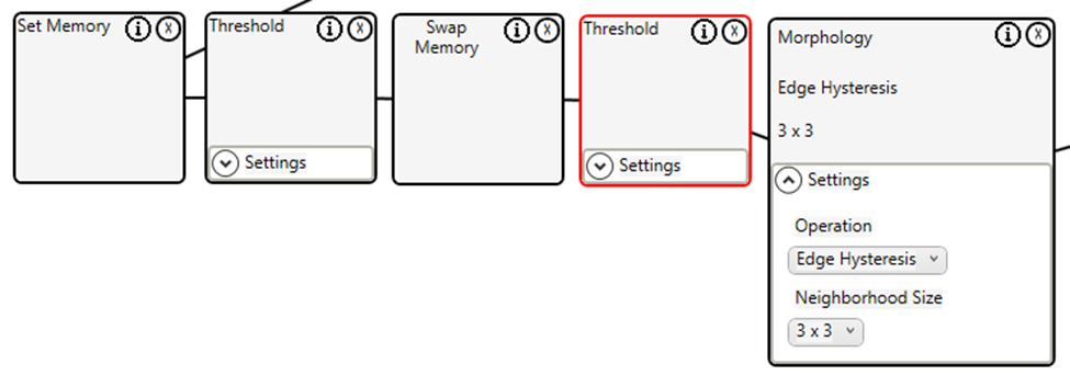
Next, we complete the Canny edge detection with double thresholding and edge hysteresis.
Finally, we use the Edge Detector to identify the most prominent lines.
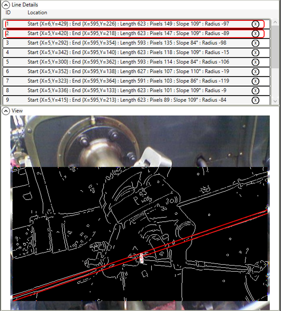
In version 3.2 of the Imaging Whiteboard a Line Detector control has been added. The line detection is performed using a Hough transform https://en.wikipedia.org/wiki/Hough_transform . The lines detected are defined by the shortest distance from the origin to the line, and the angle between the x axis and the line connecting the origin to the closest point on the line. Theoretically the lines are infinitely long.
Since we want to be able to restrict the Hough transform to a specified region we want to display the detected lines in that region. Without line length restriction the display would look like:
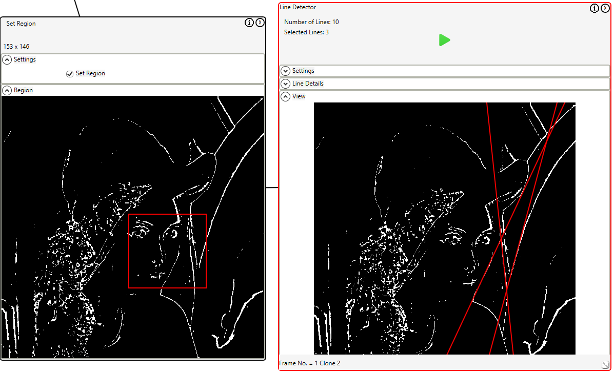
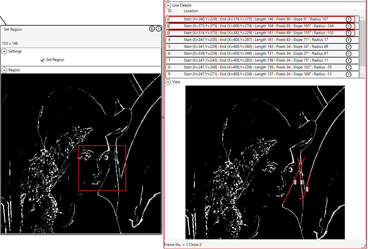
With lines restricted to the specified region the display correctly looks like:
How is this performed? Every point on a line is defined by:

where r is the distance from the origin to the closest point on the straight line, and θ is the angle between the x axis and the line connecting the origin with that closest point.
So for each line the start and end points must be trimmed to lay on the region perimeter. Each point must be trimmed horizontally and vertically. Horizontal trimming looks like:
if (point.X < region.Left)
{
point.X = region.Left;
point.Y = _centerH – (int)((radius – Math.Cos(thetaRadians) * (region.Left – _centerW)) /
Math.Sin(thetaRadians));
}
if (point.X > region.Right)
{
point.X = region.Right;
point.Y = _centerH – (int)((radius – Math.Cos(thetaRadians) * (region.Right – _centerW)) /
Math.Sin(thetaRadians));
}
Vertical trimming is similar. The _centerW and _centerH values exist because the origin is in the center of the image, but, pixel 0,0 is in the top left corner; adjustment must be made before and after the calculation.
The Imaging Whiteboard is done. I’ve added every feature I can think of, fixed every bug I know about. 3.0.5 is the final version.
So, what is the next project?
Obviously, I asked ChatGPT.
Me:
“My name is Steve Weavers; my personal web site is http://sound-analysis.com/ . I am responsible for The Musicians Workbench and The Imaging Whiteboard. I have just completed the Imaging Whiteboard. I am looking for ideas for my next project. What do you think I should tackle?”
Here is what it said:
“Hi Steve! It’s great to hear that you’ve completed the Imaging Whiteboard. As for your next project, there are many directions you could go in. Here are a few ideas to consider:
Music notation software: If you enjoy working on music-related projects, creating a software tool that makes it easier for musicians to notate their compositions could be a valuable resource for the community.
Audio editing software: Building an audio editing software could be a complex but rewarding project. You could focus on a specific niche, such as podcast editing, or create a comprehensive tool that covers all aspects of audio editing.
Virtual instrument plugin: If you have experience with music production software, developing a virtual instrument plugin could be a fun challenge. This could involve creating realistic-sounding emulations of real instruments, or coming up with entirely new and unique sounds.
Music recommendation engine: With so much music available online, it can be overwhelming for listeners to discover new artists and albums. Creating a recommendation engine that uses machine learning algorithms to suggest music based on a user’s listening history could be a valuable tool for music lovers.
Audio analysis tool: Given your background in sound analysis, creating a tool that helps users analyze audio files could be a natural fit. This could involve developing algorithms to identify key features of the audio, such as tempo, key, and tonality.
I hope these ideas give you some inspiration for your next project!”
Me:
“Those were excellent suggestions. Do you have any ideas for imaging projects?”
“Certainly, here are some ideas for imaging projects you could consider:
Image recognition software: Developing software that uses machine learning algorithms to recognize and identify objects within images could be a valuable tool for a range of industries, from healthcare to security.
Image processing software: Creating software that enhances or alters images could be a fun and creative project. You could focus on specific effects, such as color correction or noise reduction, or create a comprehensive tool that covers a range of editing capabilities.
Virtual reality experiences: With the increasing popularity of virtual reality technology, creating immersive visual experiences could be a rewarding project. This could involve creating 360-degree images or videos, or developing interactive VR games.
Image compression algorithms: Developing algorithms to compress image files without compromising their quality could be a valuable resource for a range of industries, from web development to photography.
Augmented reality applications: Building applications that overlay virtual objects or information onto real-world images could be a fun and innovative project. This could involve creating educational tools or marketing applications for businesses.
I hope these ideas provide some inspiration for your next imaging project!”
That’s brilliant! The Audio analysis tool might be a good challenge. What do you think?
Using the MNIST database of handwritten digits MNIST database – Wikipedia a convolutional neural network was trained to an accuracy of 90%. This took 50 epochs.

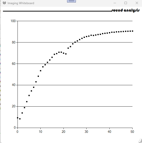
The trained model was loaded into the Image Classifier control and used to identify handwritten digits.
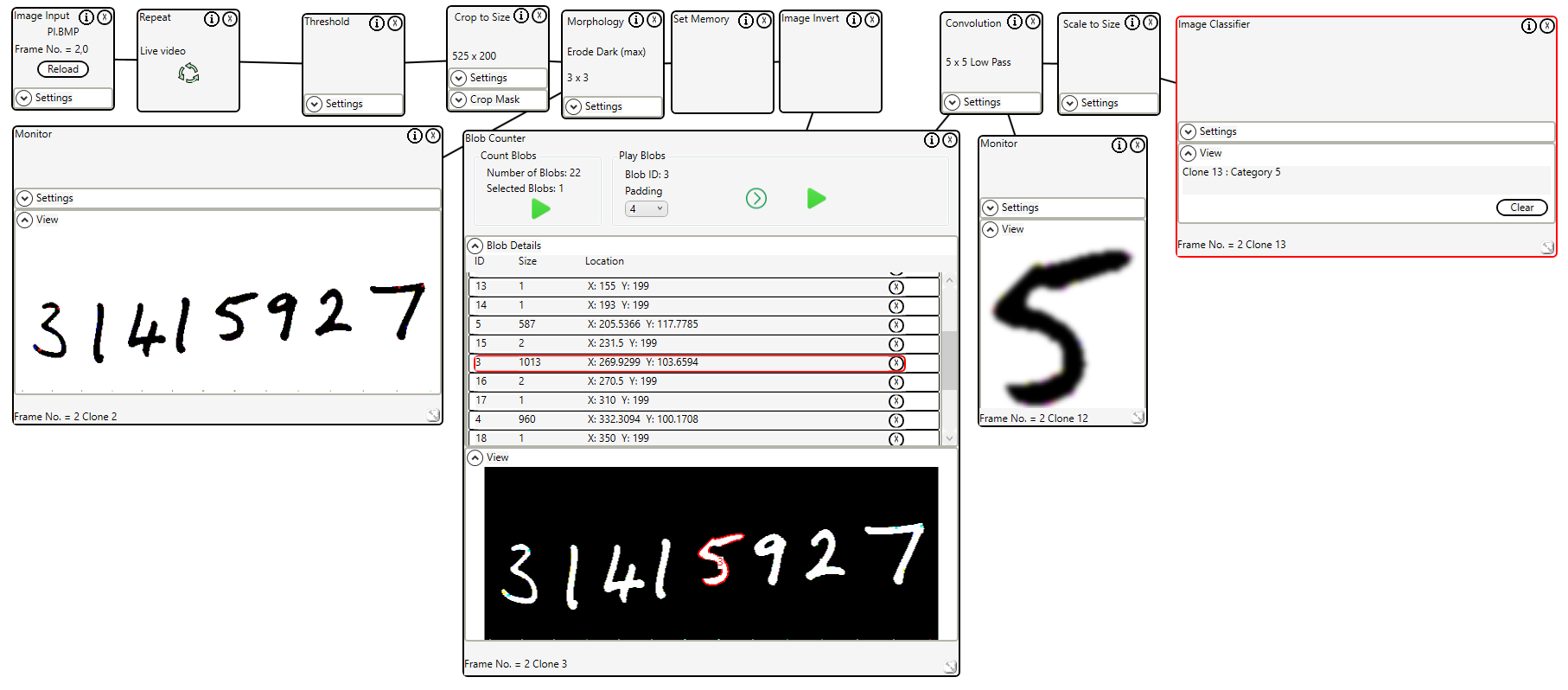
The files required to reproduce this demo are available here https://drive.google.com/file/d/1XKSYvJfAW1maNsaiV0iaWZXor0Tbtuat/view?usp=share_link
The new blob counter control in the Imaging Whiteboard (2.5.7) can be used for more advanced image analysis algorithms.
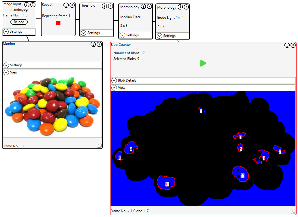
Here we see an image of M&Ms and we want to know how many blue ones are visible. The threshold control is used to separate the blue component of the image. The morphology controls are used to filter out spurious noise and partially visible M&Ms. The blob counter will identify the blobs and allow the user to select the blobs or interest. The selected blobs count is the answer.

Here we can see the results of two methods applied to the same image shown on the monitor simultaneously. The split screen feature will be available in version 2.5 of the Imaging Whiteboard.
Noise is added to the image and the set memory control will write the noisy image to the secondary memory. The temporal filter is applied to the primary memory. Swap memory switches the primary and secondary memories. The 3×3 median filter is applied. The monitor shows the primary image (morphology result) on the left, and the secondary (temporal filter) on the right.
White noise will contain all frequencies. By applying filters to white noise and viewing the resulting spectrum the effects can be viewed. Here we see the test signal generator producing white noise on 2 channels and the resulting spectrum. The high pass filter is applied to the signal and the resulting spectrum with low frequencies eliminated is shown. The low pass filter is then applied eliminating the high frequencies.
