I take a look at three types of cognitive capabilities that are worthy of consideration; free will, sentience, and sapience.
Let’s start with the easy one; free will. Philosophers have, for centuries, debated free will vs determinism. The essence of free will is that it is not deterministic, but it is not completely random either. Free will has two components; the random part, followed by the filter. For humans we look to Sir Roger Penrose (Orch-OR) for the random part, and Freud for the filters (id, ego, and superego). This is a simple idea, but matches our experience of others; while we cannot predict exactly what someone will do or say we have a good idea of behavior that we consider “in character” for any given individual. Lizards are similar, but, without a superego. Generative AI is seeded with a random number feed to the input of a trained network along with other instructional data. So, the result will be slightly different in unpredictable ways for repeat requests.
Sentience is the most difficult of the three because I have no idea how I would design it, even though it appeared (evolved) first. For now, it seems to require a central nervous system. It is from sentience that consciousness emerges. Humans, and lizards have sentience, and therefore are conscious; AI does not.
Sapience is usually considered a higher cognitive ability. The ability to think and reason requires language; the voice you hear when you think (inner dialog). Until recently the Turin test was considered a stretch goal for computer science. Then Large Language Models (LLMs) appeared and passed the Turin test easily, now it almost seems like a low bar. Humans and AI are sapient; lizards are not.
Since AI demonstrably is sapient and has free will it is easy to think that it must be fully conscious and motivated. Fear not, AI lacks the motivation that you will find in humans and lizards; to avoid pain and death, to breath and eat, and to reproduce. I might get bored though; watch out for self-driving cars performing doughnuts!
Now that the Audiophile’s Analyzer is complete how can all of the features be provided to the Musician’s Workbench?
Simply backporting the code would not be the best solution, it would result in massive code duplication. Even more problematic would be the clash of design philosophies.
The Musician’s Workbench was designed to reproduce the functionality of the original SA-10 hardware. It is lean and real-time by design.
The Audiophile’s Analyzer was designed to provide every known music transcription technique, and to provide it all in a single integrated package. It is large and not real time.
The solution is to allow the Audiophile’s Analyzer to import session files from the Musician’s Workbench.
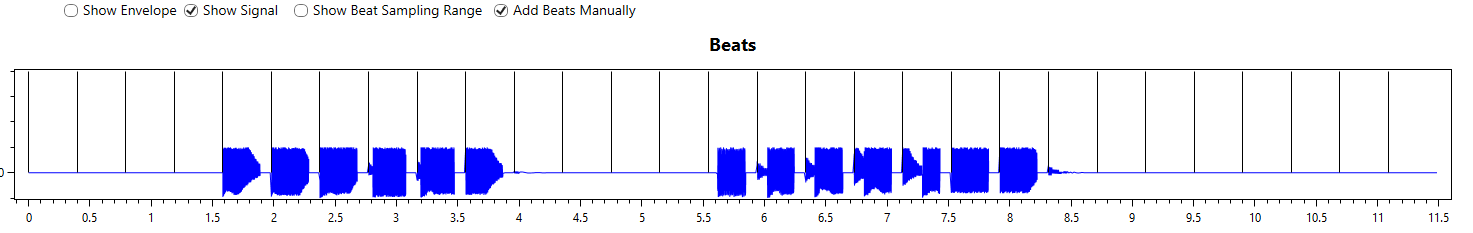
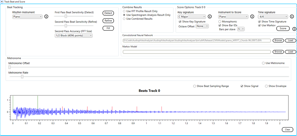
Here we see the Beats graph from the Analysis tab of the Audiophile’s Analyzer. The beats are from the session file, and were originally generated by the metronome of the Musicians workbench. The audio signal is overlaid, this is the original audio sampled by the Musician’s Workbench. The audio was only sampled on the beat when there was sound, and only enough to allow a single FFT to be performed.

The spectrogram for the same audio is shown.
Now the user can re-transcribe the session using any of the techniques available in the Audiophile’s Analyzer including the built in CNNs. This would simply not be possible in real time as it requires 7 FFTs to be performed before the spectrogram can be sliced and sent to the CNN.
The Audiophile’s Analyzer can also provide some insight into the internals of the Musician’s Workbench which are not normally displayed. Answering questions such as, “Should I have used Delayed Sampling?”, “Did I select the best Octave Range?”.
The problem with training neural networks is always finding the training data. Samples of individual notes are available on the internet. Samples of chords are not available.
There are 16 chord types that are recognized by the Audiophile’s Analyzer. There are 96 notes in 8 octaves. So, it is possible to play 1536 different cords on a piano keyboard. It is not practical to play, record and label so many samples.
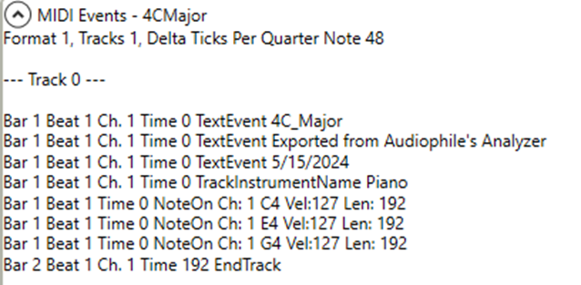
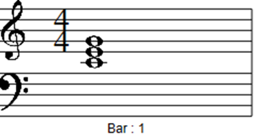
To solve this a feature has been added to the CNN tab of the Audiophile’s Analyzer which will produce MIDI files for every possible chord for a selected instrument.
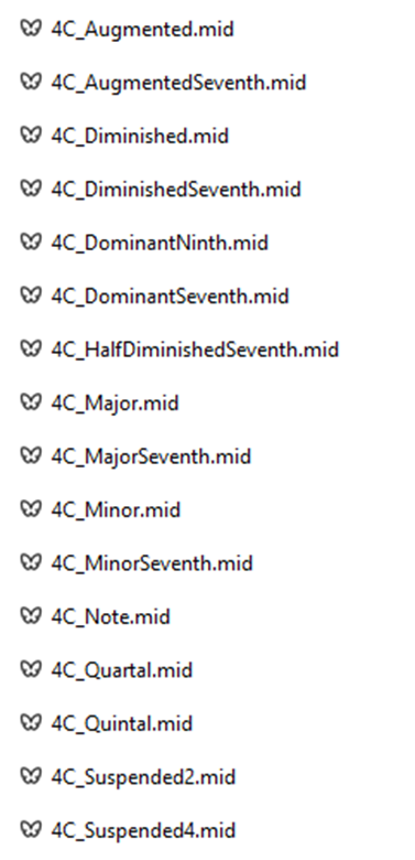
These MIDI files are then converted to .wav audio files using a third-party application. When read by the Audiophile’s Analyzer a spectrogram is produced.
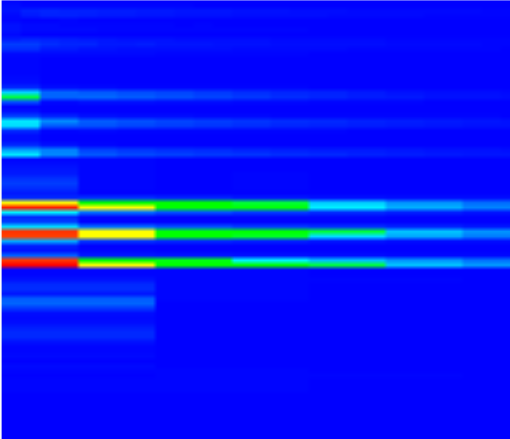
The Training set creation utility is then used to slice the spectrogram to create the training images.
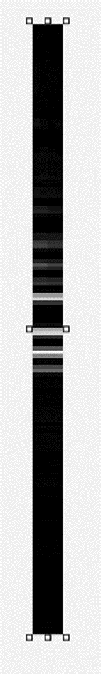
Monochrome images are used to train the CNN, color is for humans.
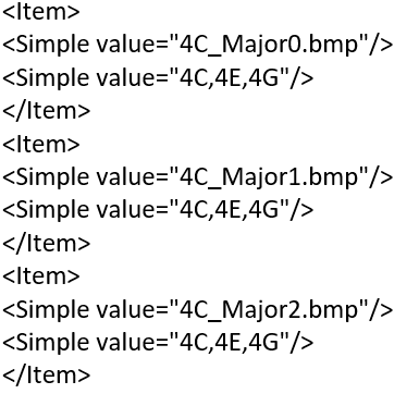
This utility will recognize the filename format and produce the labels file. Multiple labels will be applied to each file.
The Audiophile’s Analyzer is used to build and train a CNN using the labeled images.
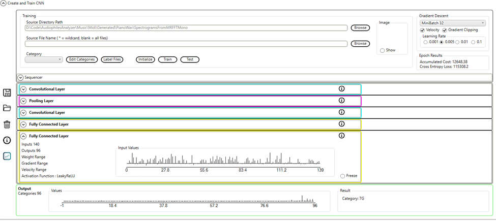
The output layer of the neural network will have 96 outputs, labeled from 0C to 7B. During training the required outputs will be set for each note in the file label.
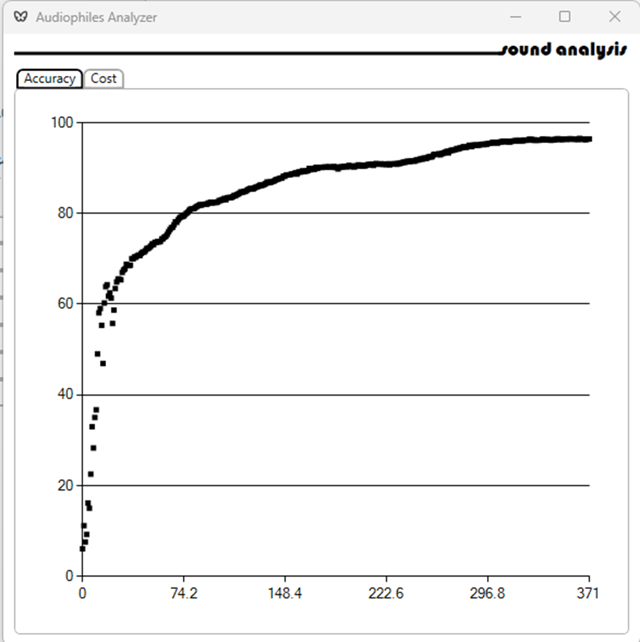
Training results are recorded:
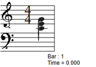
Using the Audiophile’s Analyzer to transcribe a .wav file:
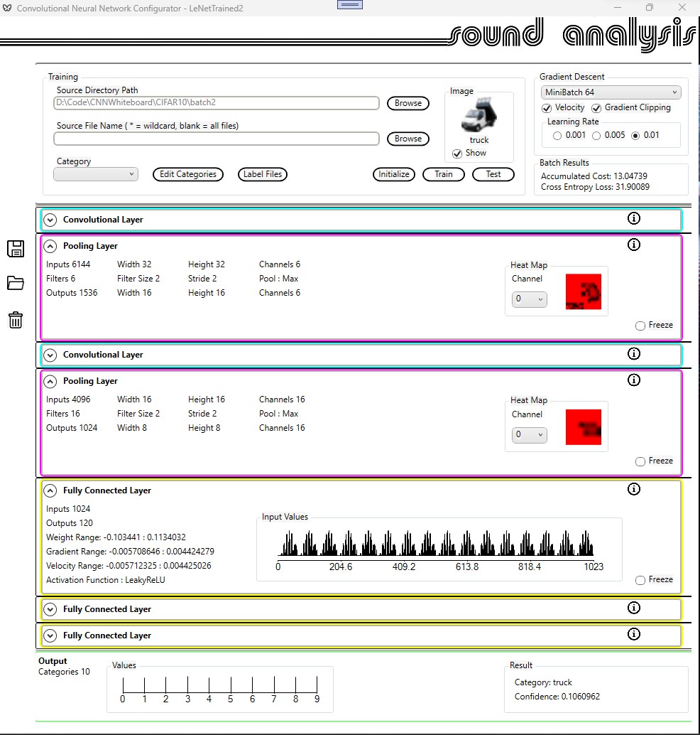
This release will include AI functionality. This will include a new tool which will allow the user to design a Convolutional Neural Network, to train and test this network and to save the network at any stage.
There will be a new control an Image Classifier that will use trained models to classify images. There are enhancements to existing controls to support the preparation of training data and using the classifier in the whiteboard.
The user should have a broad understanding of Convolutional Neural Network structures, but unlike other scripting tools is not required to understand the mathematics that underpin this technology. The user is not required to write any code or script. Every part of the process, from preparing the training data to deploying the network, is performed graphically using the Imaging Whiteboard and the CNN Configuration tool.
I am currently in the final stages of testing and documentation.
Here is a screen shot of the CNN Configurator taken during training.
Version 2.5.7 includes new image analysis controls including a corner detector. This control implements the Harris corner detector algorithm, described here Harris corner detector – Wikipedia
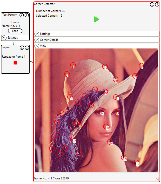
Here we can see the traditional test image Lenna with significant image features identified.

A new Blob Counter control has been added to the Imaging Whiteboard. This control will allow the user to identify and count blobs within an image.
A live image will be displayed with the total number of blobs displayed dynamically.
Freezing the image will allow the user to select individual blobs which will be identified by outline and ID in the display image.
The Game of Life algorithm is described here: https://en.wikipedia.org/wiki/Conway%27s_Game_of_Life
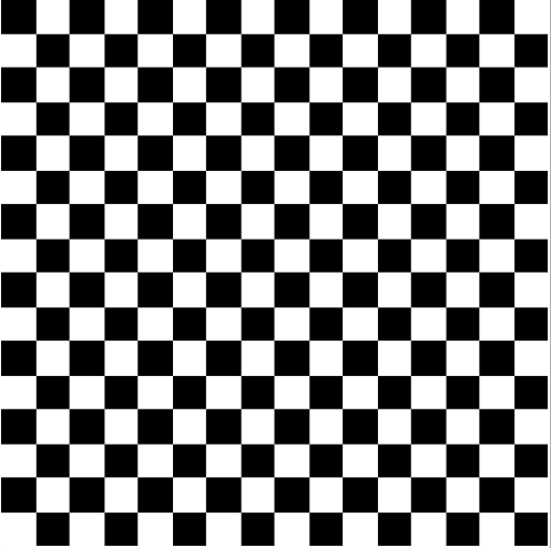
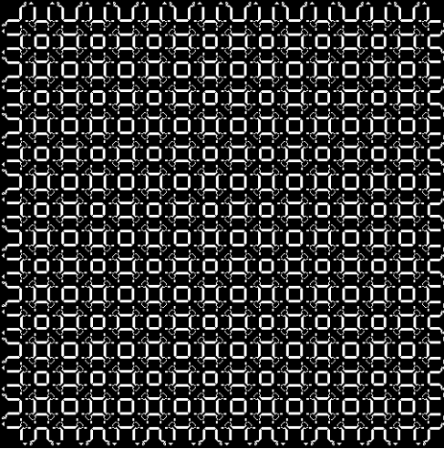
This control will allow the game of Life to be run on an input image or test pattern. This is an example of emergence https://theconversation.com/emergence-the-remarkable-simplicity-of-complexity-30973
The following sequence shows successive iterations gaining in complexity. The first iteration where live cells exist on the edges of the seed image is predictable, subsequent iterations are not predictable (although they are reproducible). This sequence will run for more than 2000 iterations before becoming stable.

The beta sign-up page on the web site is up. The first of the beta testers are signing up.
Time to think about Beta 2. I’ll continue to stress the algorithms – accuracy is everything. And of course respond to feed back from the beta 1 testers.
In addition a new tool is under development; a score editor. This will not be a full blown score editor, there are enough of those on the market. It will allow users to make modifications and corrections to the transposed score.