The Mandelbrot generator has been added to the Imaging Whiteboard. The whole point of the Mandelbrot is infinite complexity from a simple algorithm. The plot points are generated with only 5 lines of code:

                    Complex z = new Complex(0.0, 0.0);
                    Complex c = new Complex(((double)w - MandelbrotSize / 2 + 
                                             HOffsetSliderValue) / (ZoomSliderValue * 64), 
                                            ((double)h - MandelbrotSize / 2 + 
                                             VOffsetSliderValue) / (ZoomSliderValue * 64));
                    uint iteration = 0;
                    for (; iteration < maxIterations && z.Magnitude < 2; iteration++)
                    {
                        z = (z * z) + c;
                    }

The control allows the user to zoom into details of the Mandelbrot and generate details.

The detail shown above is from the very left tip of the full scan. It seems that this detail repeats the full scan, but, not exactly. At first glance the Mandelbrot seems to contain much repetition; unlike fractals these repetitions are not exact.

The full un-zoomed plot looks like:

If you take a 3-dimensional object, rotate it 180 degrees in each of 3 dimensions in turn, the object will return to it’s original position.

I don’t know of an elegant mathematical proof of this; it would require the use of 3D complex numbers which do not exist (see the previous blog post ‘Using complex arithmetic to perform combination warps‘). There is an abundance of empirical evidence though.

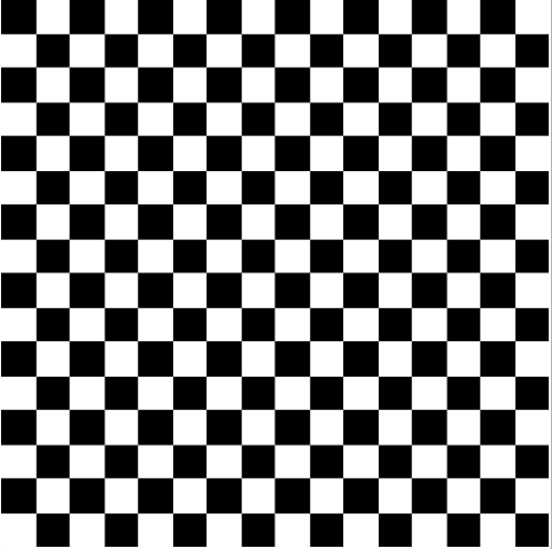
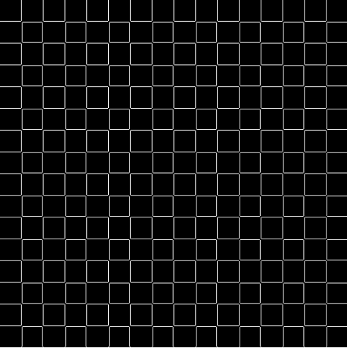
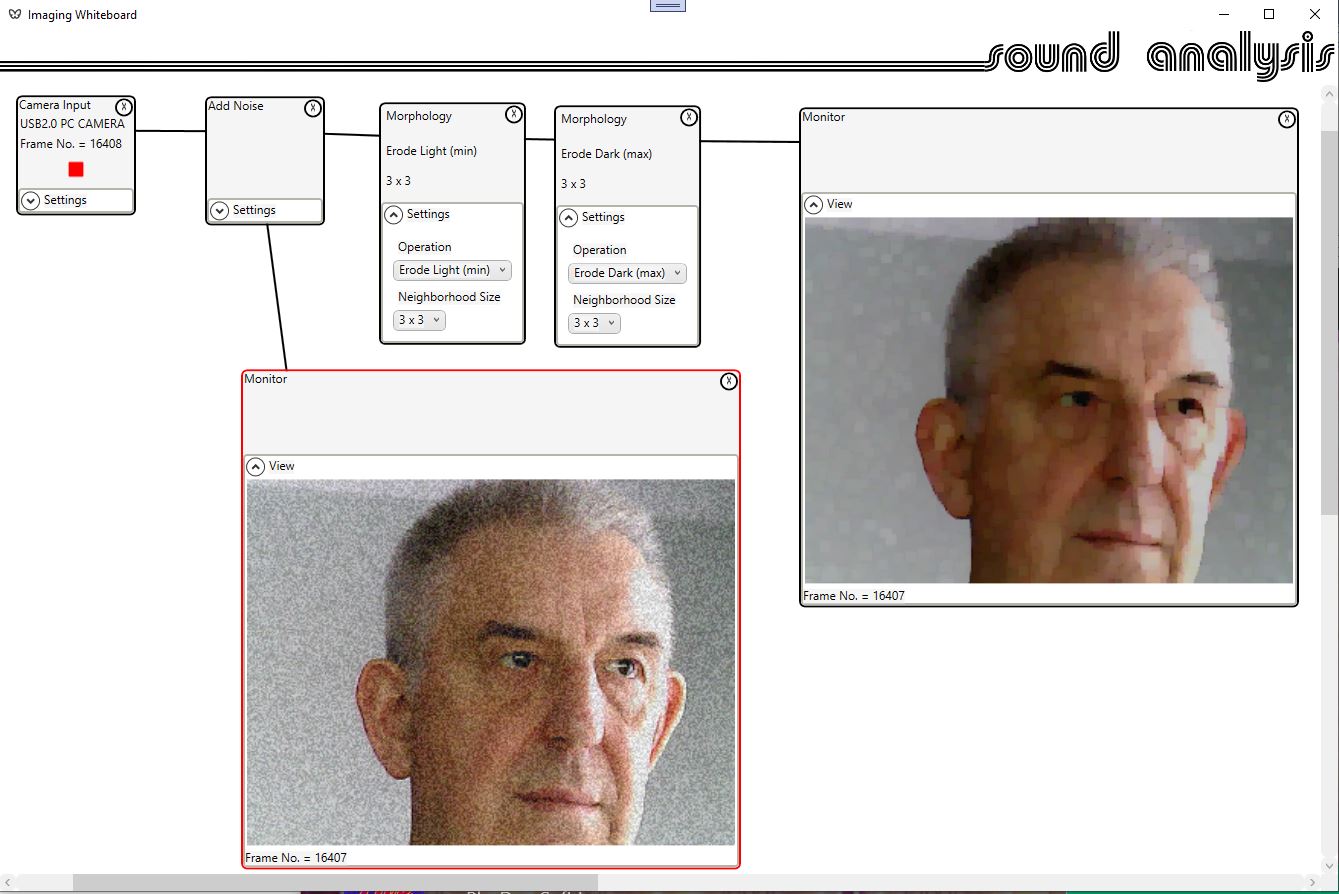
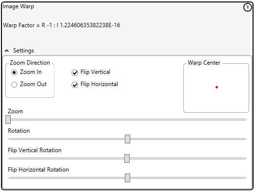
Using the warp control of the Imaging Whiteboard we can perform this 3D transformation.

Flip Vertical, Flip Horizontal, and rotate 180 degrees. The image will return to it’s original not warped position.

So if I am using regular 2D complex numbers to perform the warp, how do I perform 3D warping?

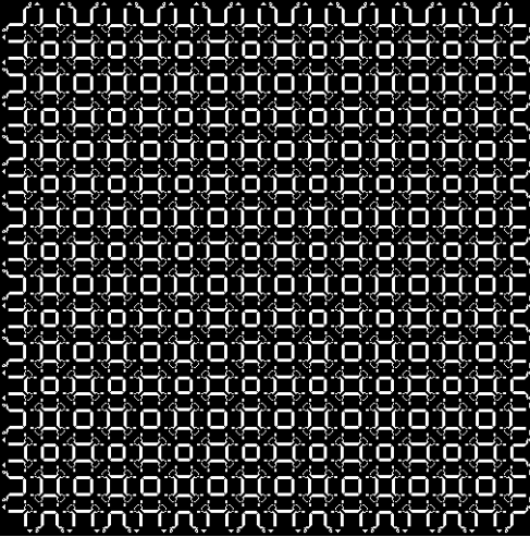
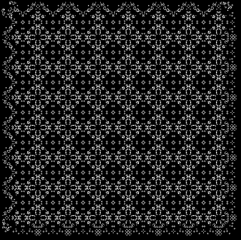
To better explain this I have created a proof of concept that implements full horizontal and vertical rotation. This is not published (I’m not sure that it is useful).

After applying the warp factor:

sourceAddress = targetAddress * WarpFactor;

The result is modified:

sourceAddress.Real = sourceAddress.Real  / Math.Cos(fhRadians);  //Horizontal rotation

sourceAddress.Imag = sourceAddress.Imag  / Math.Cos(fvRadians);  //Vertical rotation

Manipulating the real and imaginary components is not really a correct use of complex numbers

Warps are generally backward mapped, that is for each pixel in the target image the address of the required pixel in the source image is calculated. Usually co-ordinate geometry is used to calculate the source address.

In the Imaging Whiteboard complex number arithmetic is used. The code to calculate the source pixel becomes:

sourceAddress = targetAddress * WarpFactor;

Yup that is the code!

The trick is to calculate the warp factor.

No warp is (1, 0), here the source is equal to the target address.

Zoom becomes (zoom, 0).

Rotation becomes (Cos (radians), Sin (radians))

So zoom and rotate becomes (zoom, 0) * (Cos (radians), Sin (radians))

Once the warp factor is calculated the warp is almost trivial!

If it’s that easy, why not use a three dimensional complex number to perform a time warp on a captured sequence? That could be fun.

Not so fast, according to the laws of mathematics there is no such thing as a 3 dimensional complex number. 2 sure, 4 OK, even 8.

So, use 4 dimensional complex numbers (quaternions) and ignore one dimension. Turns out that will not work either, mathematics is not so easily fooled.

So I could use co-ordinate geometry, which would be horribly slow and complicated. Or just introduce a DVR control, which is what anybody else would do. The DVR control solution would be limited in its functionality i.e. the same time would have to be applied to all pixels in a frame before the image warp.

None of this is very practical as the memory requirements would be prohibitive.

If you really want to know how to do a time warp you should watch this video.  TimeWarp

The Imaging Whiteboard Users Guide has a screen shot that shows how the threshold control can be used to separate the color components of an image.

Of course once separated the color components can be processed.

This screen shot shows how the FFT filter can be applied to the green component of the checkerboard test pattern.

Note that the FFT result is also shown as green. (Click image for a better view)