The Imaging Whiteboard is done. I’ve added every feature I can think of, fixed every bug I know about. 3.0.5 is the final version.
So, what is the next project?
Obviously, I asked ChatGPT.
Me:
“My name is Steve Weavers; my personal web site is http://sound-analysis.com/ . I am responsible for The Musicians Workbench and The Imaging Whiteboard. I have just completed the Imaging Whiteboard. I am looking for ideas for my next project. What do you think I should tackle?”
Here is what it said:
“Hi Steve! It’s great to hear that you’ve completed the Imaging Whiteboard. As for your next project, there are many directions you could go in. Here are a few ideas to consider:
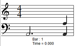
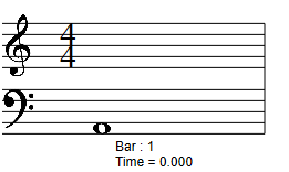
Music notation software: If you enjoy working on music-related projects, creating a software tool that makes it easier for musicians to notate their compositions could be a valuable resource for the community.
Audio editing software: Building an audio editing software could be a complex but rewarding project. You could focus on a specific niche, such as podcast editing, or create a comprehensive tool that covers all aspects of audio editing.
Virtual instrument plugin: If you have experience with music production software, developing a virtual instrument plugin could be a fun challenge. This could involve creating realistic-sounding emulations of real instruments, or coming up with entirely new and unique sounds.
Music recommendation engine: With so much music available online, it can be overwhelming for listeners to discover new artists and albums. Creating a recommendation engine that uses machine learning algorithms to suggest music based on a user’s listening history could be a valuable tool for music lovers.
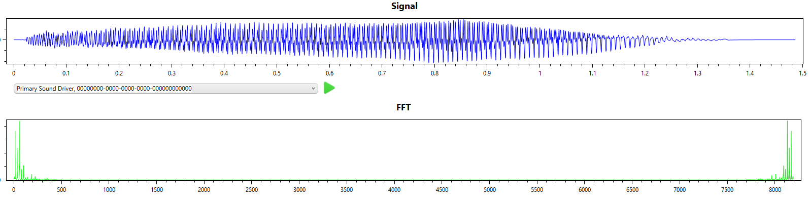
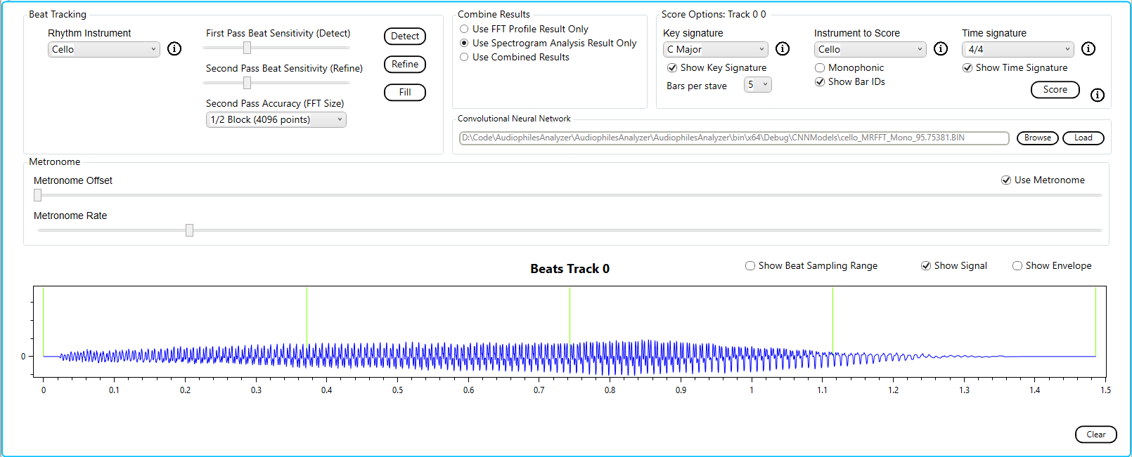
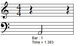
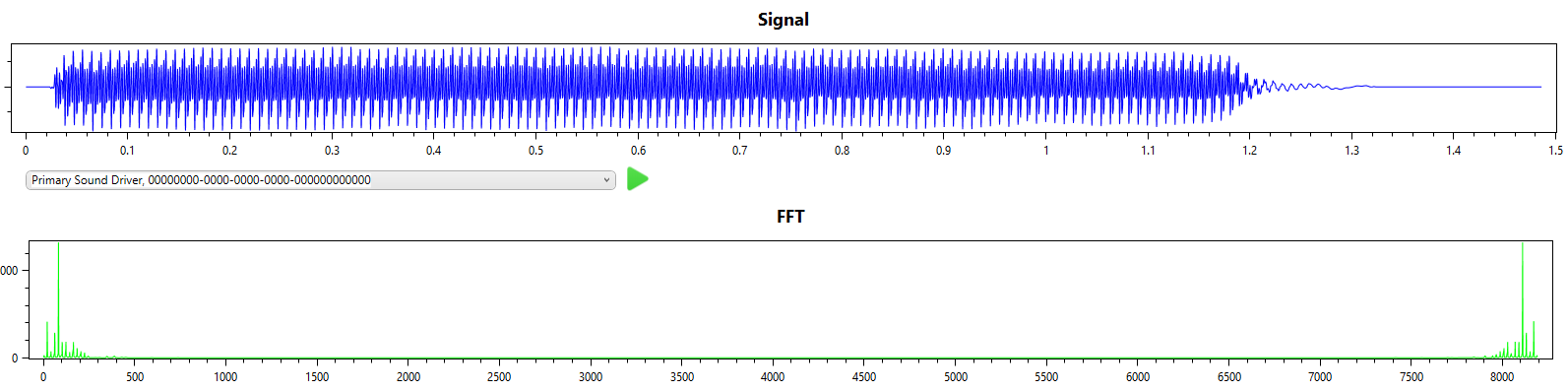
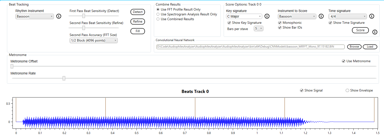
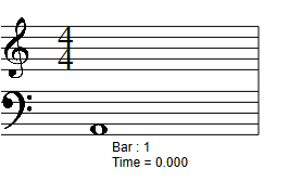
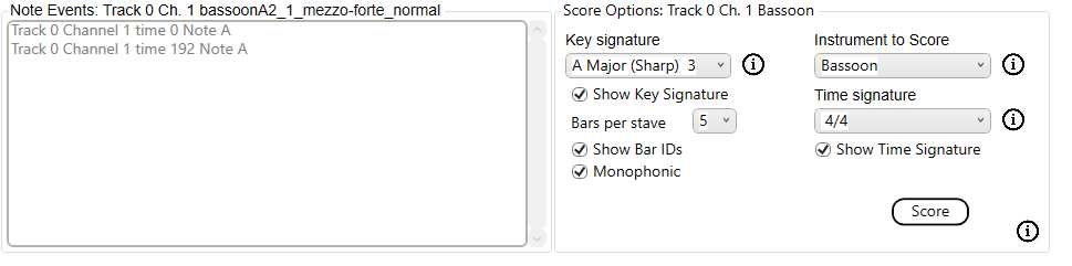
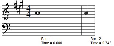
Audio analysis tool: Given your background in sound analysis, creating a tool that helps users analyze audio files could be a natural fit. This could involve developing algorithms to identify key features of the audio, such as tempo, key, and tonality.
I hope these ideas give you some inspiration for your next project!”
Me:
“Those were excellent suggestions. Do you have any ideas for imaging projects?”
“Certainly, here are some ideas for imaging projects you could consider:
Image recognition software: Developing software that uses machine learning algorithms to recognize and identify objects within images could be a valuable tool for a range of industries, from healthcare to security.
Image processing software: Creating software that enhances or alters images could be a fun and creative project. You could focus on specific effects, such as color correction or noise reduction, or create a comprehensive tool that covers a range of editing capabilities.
Virtual reality experiences: With the increasing popularity of virtual reality technology, creating immersive visual experiences could be a rewarding project. This could involve creating 360-degree images or videos, or developing interactive VR games.
Image compression algorithms: Developing algorithms to compress image files without compromising their quality could be a valuable resource for a range of industries, from web development to photography.
Augmented reality applications: Building applications that overlay virtual objects or information onto real-world images could be a fun and innovative project. This could involve creating educational tools or marketing applications for businesses.
I hope these ideas provide some inspiration for your next imaging project!”
That’s brilliant! The Audio analysis tool might be a good challenge. What do you think?